How Neural Networks Really Work: Study Notes
How Neural Networks Really Work: Study Notes
Original notebook: How does a neural net really work?
A neural network is, mathematically, a function. For a standard neural network, this function does roughly three things:
- Multiply inputs by some values, called parameters.
- Add the results together.
- Replace negative values with zero, then produce the output.
That is what one neural-network “layer” does. The same process is repeated, using the output of one layer as the input to the next. At the beginning, the parameters are usually random numbers, so an initial neural network cannot do anything useful. It is random.
To make this mathematical function learn, we need better parameters. That is where gradient descent comes in.
Start With A Simple Function
from ipywidgets import interact
from fastai.basics import *

plt.rc('figure', dpi=90)

def plot_function(f, title=None, min=-2.1, max=2.1, color='r', ylim=None):
    x = torch.linspace(min,max, 100)[:,None]
    if ylim: plt.ylim(ylim)
    plt.plot(x, f(x), color)
    if title is not None: plt.title(title)

def f(x): return 3*x**2 + 2*x + 1

plot_function(f, "$3x^2 + 2x + 1$")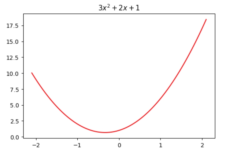
This is a quadratic function. Next, define a generic quadratic function quad with three parameters, a, b, and c. Then use Python’s partial to create mk_quad, so the resulting function only needs x as input:
def quad(a, b, c, x): return a*x**2 + b*x + c

def mk_quad(a,b,c): return partial(quad, a,b,c)

f2 = mk_quad(3,2,1)
plot_function(f2)
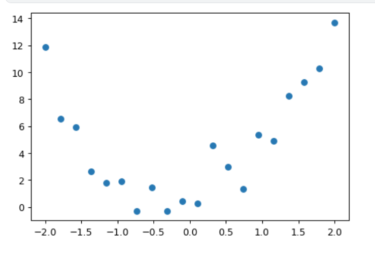
Now generate some simulated data and add noise. From the add_noise function, x and y should still roughly follow a quadratic relationship, but the random noise makes the data more realistic. Later, we will infer the parameters of the quadratic function from this data.
def noise(x, scale): return np.random.normal(scale=scale, size=x.shape)

def add_noise(x, mult, add): return x * (1+noise(x,mult)) + noise(x,add)

np.random.seed(42)

x = torch.linspace(-2, 2, steps=20)[:,None]
y = add_noise(f(x), 0.15, 1.5)

x[:5],y[:5]

output:
(tensor([[-2.0000],
         [-1.7895],
         [-1.5789],
         [-1.3684],
         [-1.1579]]),
 tensor([[11.8690],
         [ 6.5433],
         [ 5.9396],
         [ 2.6304],
         [ 1.7947]], dtype=torch.float64))
The data distribution looks like a noisy quadratic curve:
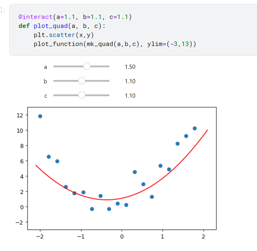
One way to fit it is to try a few values for a, b, and c, then check whether the result looks right. In this simple example, the notebook lets us interactively adjust the three parameters and observe how well the curve fits the data.
After several attempts, you can see how each parameter affects the curve: a controls how wide the parabola opens and in which direction, b changes its tilt, and c moves it up and down.
But visual judgment is not enough. We need a metric. A simple option is to measure the distance between each point and the curve:
def mae(preds, acts): return (torch.abs(preds-acts)).mean()

@interact(a=1.1, b=1.1, c=1.1)
def plot_quad(a, b, c):
    f = mk_quad(a,b,c)
    plt.scatter(x,y)
    loss = mae(f(x), y)
    plot_function(f, ylim=(-3,12), title=f"MAE: {loss:.2f}")
This updates the interactive plot by showing the current MAE, or mean absolute error, at the top.
Automatic Gradient Descent
Modern neural networks often contain tens of millions of parameters. We cannot manually adjust sliders and inspect the result. The process must be automated. Fortunately, calculus gives us a way.
The idea is simple: if we know the gradient of the MAE with respect to parameters a, b, and c, then we know how changing each parameter affects the loss. If a has a negative gradient, increasing a reduces the MAE. Since the goal is to make MAE as small as possible, that tells us which direction to move.
So we compute the gradients for all parameters, then move them a small step in the right direction.
def quad_mae(params):
    f = mk_quad(*params)
    return mae(f(x), y)

quad_mae([1.1, 1.1, 1.1])

# tensor(2.4219, dtype=torch.float64)
This output is the same as calling mae directly. Next:
abc = torch.tensor([1.1,1.1,1.1])

abc.requires_grad_()  # Tell PyTorch to calculate gradients for these parameters.
# tensor([1.1000, 1.1000, 1.1000], requires_grad=True)

loss = quad_mae(abc)
loss
# tensor(2.4219, dtype=torch.float64, grad_fn=<MeanBackward0>)

loss.backward()  # PyTorch calculates the gradients.

abc.grad
# tensor([-1.3529, -0.0316, -0.5000])
The gradients are negative, meaning the parameters are smaller than they should be. We can subtract the gradient multiplied by a small number, which slightly improves the result:
with torch.no_grad():
    abc -= abc.grad*0.01
    loss = quad_mae(abc)

print(f'loss={loss:.2f}')
# loss=2.40
The loss becomes smaller. The small multiplier is called the learning rate, one of the most important hyperparameters in training. The update is wrapped in torch.no_grad() because abc -= abc.grad*0.01 is not part of the quadratic model itself. We do not want PyTorch to include the update operation in the model graph.
Repeat the same steps in a loop:
for i in range(10):
    loss = quad_mae(abc)
    loss.backward()
    with torch.no_grad(): abc -= abc.grad*0.01
    print(f'step={i}; loss={loss:.2f}')

output:
step=0; loss=2.40
step=1; loss=2.36
step=2; loss=2.30
step=3; loss=2.21
step=4; loss=2.11
step=5; loss=1.98
step=6; loss=1.85
step=7; loss=1.72
step=8; loss=1.58
step=9; loss=1.46
The loss keeps decreasing. If we run more iterations, it can continue decreasing toward zero. But if training goes too far, the loss may increase again because the parameters move away from the optimum. To avoid this, the learning rate can be reduced when necessary. Most frameworks, including fastai and PyTorch, provide tools for handling learning-rate schedules.
From Quadratic Functions To Neural Networks
Neural networks can do far more than fit this simple quadratic function. In practice, neural networks have enormous expressive power and can approximate sufficiently complex computable functions. Computable functions cover many scenarios we care about: speech recognition, drawing, medical image diagnosis, fiction writing, and much more.
Compared with the simple example above, a more complex neural network still mainly does two things:
- Multiply many parameters, then add the results.
- Apply the function
max(x, 0)to turn negative values into zero.
In PyTorch, max(x, 0) can be implemented with torch.clip(x, 0.). More commonly, it is written as F.relu(x), from torch.nn.functional. In this context, ReLU is equivalent to max(x, 0).
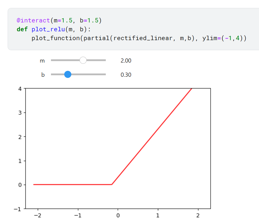
The original notebook lets us adjust m and b interactively to observe the curve:
The corresponding code:
def rectified_linear(m,b,x):
    y = m*x+b
    return torch.clip(y, 0.)

import torch.nn.functional as F
def rectified_linear2(m,b,x): return F.relu(m*x+b)
plot_function(partial(rectified_linear2, 1,1))

@interact(m=1.5, b=1.5)
def plot_relu(m, b):
    plot_function(partial(rectified_linear, m,b), ylim=(-1,4))
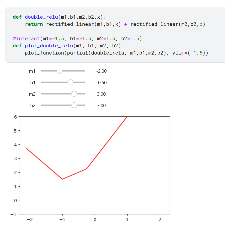
Here, m controls the slope, while b controls where the bend appears. Finally, we can combine two similar functions and adjust four parameters interactively. In theory, by stacking more functions, we can approximate more complex outputs from a single input.
Follow ZiCode on WeChat
If this post was useful, you can follow later updates on WeChat as well.

X / Twitter
Follow @ax2_zicode
Faster technical notes, short thoughts, and new-post alerts are posted on X.